Octave Installation

Octave is a software for numerical computations, the language which uses similarly like Matlab, but Octave is free.
Linux:
Avoiding to install Octave 4.0.0, during Andrew Ng do not recommend this version. It is said that that version of Octave could cause programming assignments submitting fail. We install Octave through PPA(Personal Package Archive), instead of installing from linux distribution’s software repositories.
To set up your system to install Octave:

sudo apt-add-repository ppa:octave/stable
sudo apt-get update
sudo apt-get install octave

When it done, i get a version of 4.0.2 by that time, and it works well.

Model Representation

This week we introduce multivariate linear regression and notation for equations where we can have any number of input variables.
$x^{(i)}_j$ = value of feature $j$ in the $i^{th}$ training example
$x^{(i)}$ = the column vector of all the feature inputs of the $i^{th}$ training example
$m$ = the number of training examples
$n$ = $\mid x^{(i)} \mid$; (the number of features)

Multivariate Linear Regression

Linear regression with multiple variables is also known as “multivariate linear regression”.
The multivariable form of hypothesis function accommodating these multiple features is as follows:
$h_\theta(x) = \theta_0 + \theta_1x_1 + \theta_2x_2 + \theta_3x_3 + \cdots + \theta_nx_n$
For concisely represent multivariable hypothesis function, we using the definition of matrix multiplication:
$h_\theta(x) = \begin{bmatrix} \theta_0&\theta_1&\cdots&\theta_n \end{bmatrix}$ $\begin{bmatrix} {x_0}\\ {x_1}\\ {\vdots}\\ {x_n}\\ \end{bmatrix}$ $= \theta^T x$
This is a vectorization of our hypothesis function for one training example.
Remark: Note that for convenience reasons in this course we assume $x_0^{(i)} = 1$ for $(i \in 1,…,m)$
The following example shows us the reason behind setting $x_0^{i} = 1$:
$X = \begin{bmatrix} x_0^{(1)}&x_0^{(2)}&x_0^{(3)}\\ x_1^{(1)}&x_1^{(2)}&x_1^{(3)} \end{bmatrix}$ $, \theta = $ $\begin{bmatrix} \theta_0 \\ \theta_1 \end{bmatrix}$
As a result, you can calculate the hypothesis as a vector with:
$h_\theta(X) = \theta^TX$

Gradient Descent For Multiple Variables

Repeat until convergence: {
$\theta_j := \theta_j - \alpha\frac{1}{m}\sum\limits_{i=1}^m(h_\theta(x^{(i)}) - y_j^{(i)})$ for $j := 0…n$
}

Gradient Descent in Practice I - Feature Scaling

There two techniques to help to speed up gradient descent are feature scaling and mean normalization. This is because $\theta$ will descend quickly on small ranges and slowly on large ranges, and so will oscillate inefficiently down to the optimum when the variables are very uneven. But these aren’t exact requirements.

feature scaling
Feature scaling involves dividing the input values by the range, make sure features are on a similar scale:
$x_i := \frac{x_i}{s_i}$

mean normalization
We use mean normalization to perform feature scaling. Mean normalization involves subtracting the average value for an input variable from the values for that input variable resulting in a new average value for the input variable of just zero.
$x_i := \frac{x_i - \mu_i}{s_i}$
*$\mu_i$ is the average of all the values for feature(i) and $s_i$ is the range of values(max - min), or $s_i$ is the standard deviation.

Gradient Descent in Practice I - Learning Rate

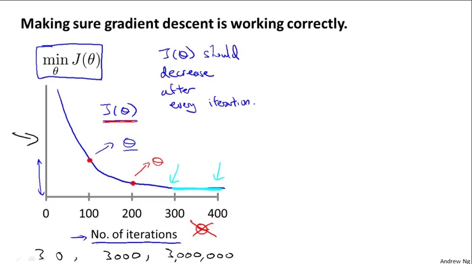
Debugging gradient descent(recommend)
Plotting a contour, which its x-axis with the number of iterations, and the cost function, $J(\theta)$ over the number of iterations of gradient descent. Make sure the gradient descent works well by visuallizing.

Automatic convergence test
Declare convergence if $J(\theta)$ decreases by less than E in one iteration, where E is some small value such as $10^{-3}$. However in practice it’s difficult to choose this threshold value.

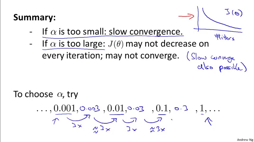
The choosing of learning rate
The learning rate $\alpha$ shouldn’t be too small, otherwise gradient descent would converge slowly.
The learning rate $\alpha$ shouldn’t be too lager neither, otherwise gradient descent would even not converge(because of overshoot problem).

Features and polynomial Regression

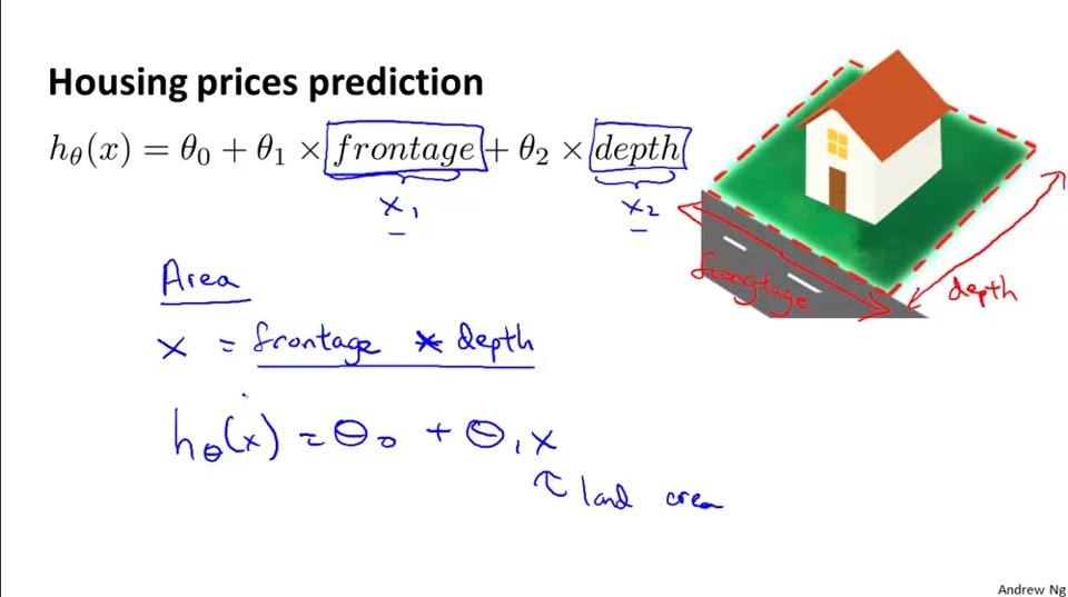
Feature reducing
Reducing features from serveral to one, such as, we substitute $x_1$ and $x_2$ with $x_3$ in the form of $x_3 = x_1 * x_2$, etc. For exmaple, the frontage of a house($x_1$) is 50 feet and the depth of the house($x_2$) is 100 feet, then the size of the house or the land area($x_3$) is 500 ${feet}^2$, we can combine $frontage$ and $depth$ into a new feature $land area$ by taking $frontage * depth$.

Polynomial Regression
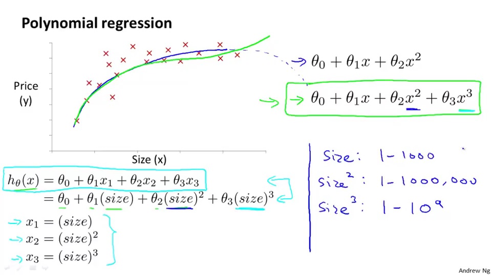
We can change the behavior or curve of our hypothesis function by making it a quadratic, cubic or square root function(or any other form), as follows:
quadratic: $h_\theta(x) = \theta_0 + \theta_1x_1 + \theta_2x_1^2$
cubic: $h_\theta(x) = \theta_0 + \theta_1x_1 + \theta_2x_1^2 + \theta_3x_1^3$
square root: $h_\theta(x) = \theta_0 + \theta_1x_1 + \theta_2\sqrt{x_1}$
pros: hypothesis function would fit the data well.
cons: range of $x_1^2$ and $x_1^3$ will increase rapidly and exponentially. Now, feature scaling becomes very important.

Normal Equation

Besides gradient descend, there is another way to minimize hypothesis function $J(\theta)$, that is normal equation.
Normal equation formula: $\theta = {(X^TX)}^{-1}X^Ty$
*There is no need to do feature scaling with the normal equation.

Comparision of gradient descent and normal equation:

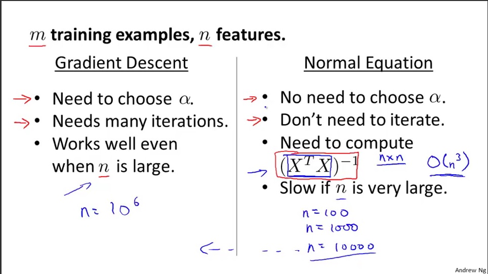
When the number of features gets so big, like, exceeds 10,000 it might be a good time to go from normal equation to gradient descent. Otherwise, we prefer to using normal equation.

Normal Equation Noninvertibility

If $X^TX$ is noninvertible, the common causes might be having:

Solutions to the above problems include deleting a feature that is linearly dependent with another or deleting one or more features when there are too many features.

Note: All materials come from Coursera Andrew Ng’s Machine Learning Class.
Acknowledgement:
Coursera
Andrew Ng

References:
http://wiki.octave.org/Octave_for_Debian_systems
https://en.wikipedia.org/wiki/Feature_scaling