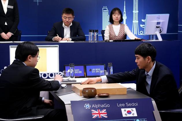
On March 19, 2016, one of the strongest Go player in the world, lee Sedol, has been defeated by Google DeepMind’s artificial-intelligence program, AlphaGo. After machine first beats mankind in 1997, again, artificial intelligence rises people’s interest. Machine learning was widely known to the public by that game, and what behind AlphaGo is an artificial neural network, a deep learning method, which deep learning is a subset of machine learning.

As an important field of Computer Science, Machine Learning nowadays become more applicable than decades ago because of enormous amount of data which generated every day by the internet or electronic devices and the powerful computational ability now we have. There are many areas have been targeted by machine learning: Data mining, Auto vechiles, Recommemdations, Healthcare, Gen engine, Market analyzing, etc. And it is changing our live right now.

Machine Learning Definition

Capability Of Machine Learning

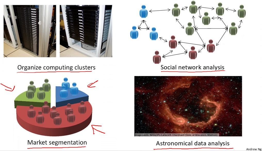
Use Cases That Using Machine Learning

Database mining.Large datasets from growth of authomation/web.
E.g., Web click data, medical records, biology, engineering.

Applications can’t program by hand
E.g., Autonomous helicopter, Handwriting recognition, most of Natural Language Processing(NLP), Computer Vision.

Self-customizing programs
E.g., Amazon, Netflix product recommendations.

Understanding human learning(brain, real AI)

Machine Learning Algorithms

Generally, machine learning algorithms are classified into two categories: Supervised learning and unsupervised learning.

Supervised Learning
In supervised learning, the output of a bunch of data set have been well and correctly labeled, letting the algorithm to find the relationship between the input and the output.

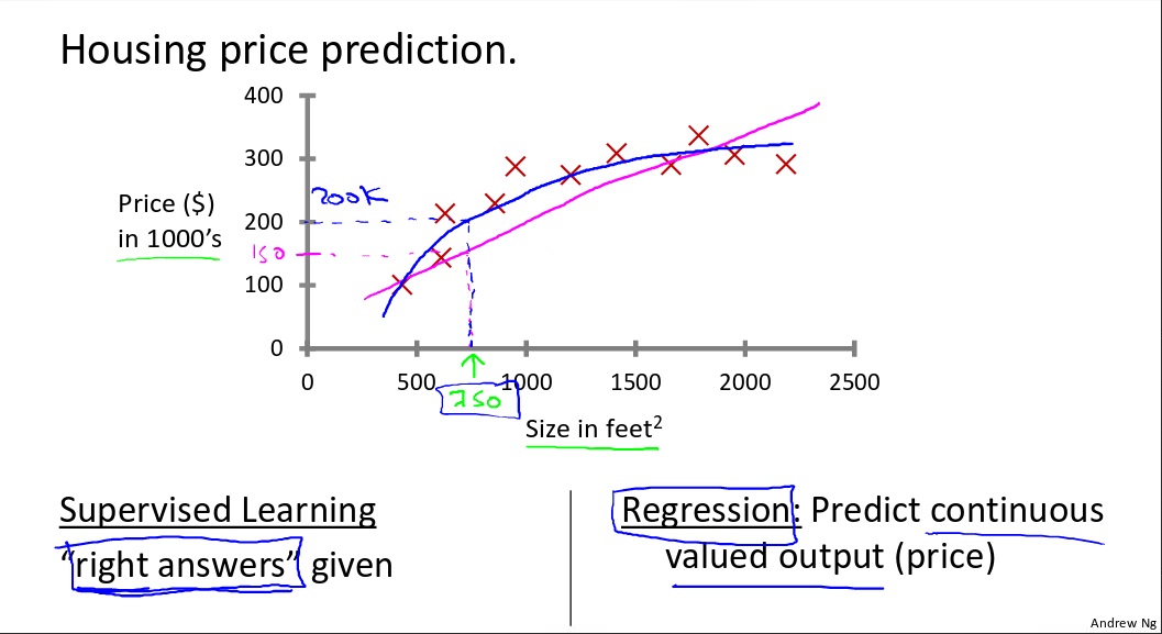
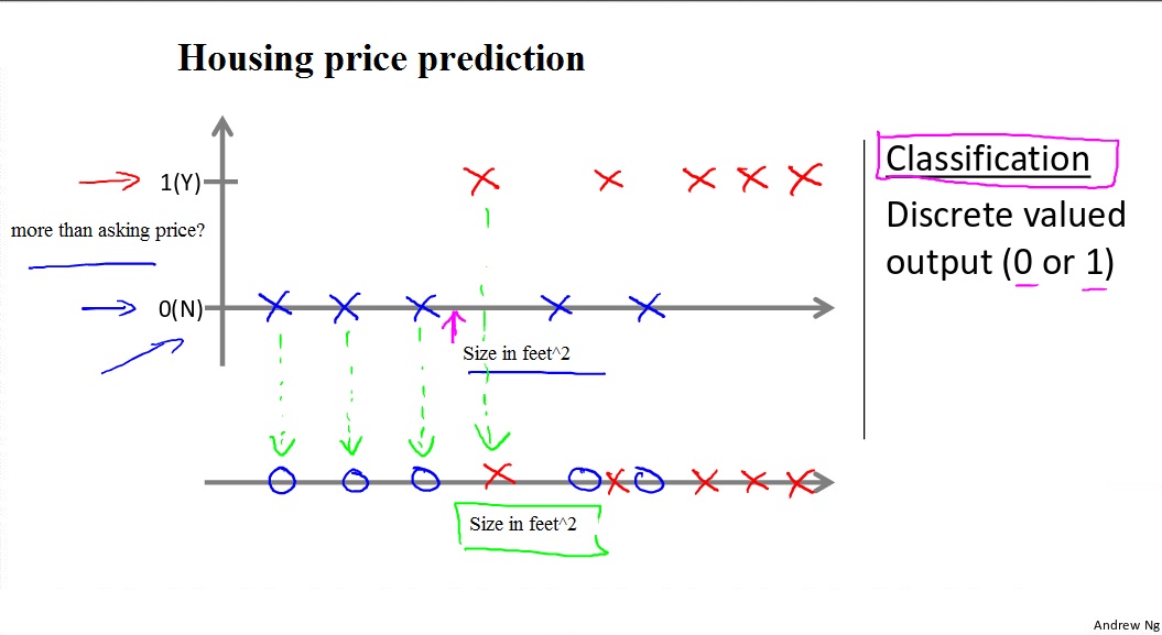
Regression and Classification are two important components of supervised learning. In a regression problem, we are trying to predict within a continuous output, meaning that we are trying to map input variables to some continuous function. In a classification problem, we are instead trying to predict results in a discrete output. In other words, we are trying to map input variables into discrete categories.

Example:
Given data about the size of houses on the real estate market, try to predict their price. Price as a function of size is a continuous output, so this is a regression problem.

We could turn this example into a classification problem by instead making our output about whether the house “sells for more or less than the asking price.” Here we are classifying the houses based on price into two discrete categories.

Unsupervised Learning
Unsupervised learning allows us to approach problems with little or no idea what our results should look like. We can derive structure from data where we don’t necessarily know the effect of the variable. We can derive this structure by clustering the data based on relationships among the variables in the data.

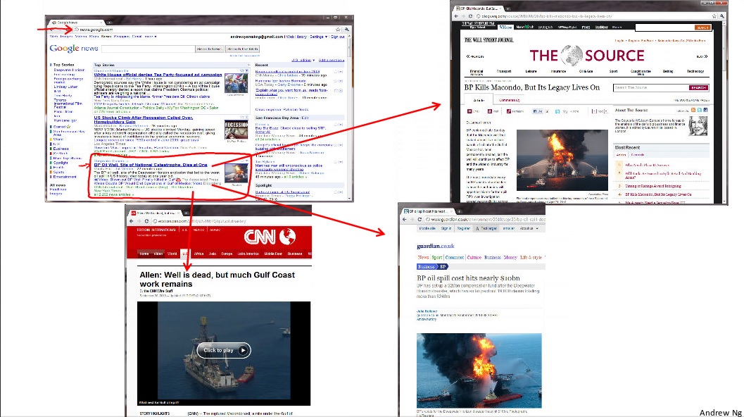
In other words, letting a algorithm to find the commons or patterns among all these variables in the data. Clustering is putting data together which have common features, Non-clustering is discrete data into two or more groups by the group’s own feature.

Example:
Clustering: Take a collection of 1,000,000 different genes, and find a way to automatically group these genes into groups that are somehow similar or related by different variables, such as lifespan, location, roles, and so on.

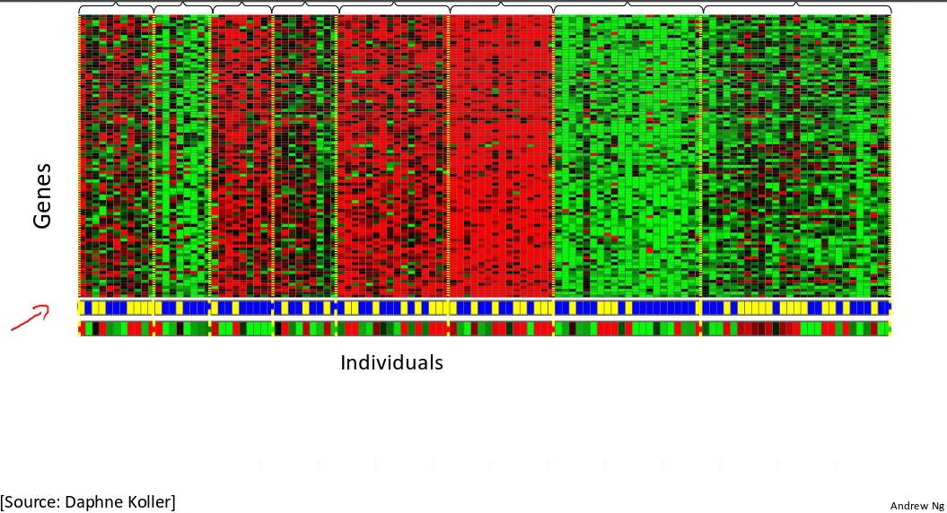
Non-clustering: The “Cocktail Party Algorithm”, allows you to find structure in a chaotic environment.(i.e. identifying individual voices and music from a mesh of sounds as a cocktail party).
Cocktail party problem algorithm: [W,s,v] = svd((repmat(sum(x.x,1),size(x,1),1).x)*x’);

Model Representation

$x^{(i)}$ denotes the “input” variables
$y^{(i)}$ denotes the “output” or target variables that we are trying to predict.
$(x^{(i)},y^{(i)})$ denotes a training example.
$(x^{(i)},y^{(i)})$; i=1,…,m denotes a list of m training examples.

• Note that the superscript “(i)” in the notation is simply an index into the training set, and has nothing to do with exponentiation.

X denotes the space of input values.
Y denotes the space of output values.
Most situations, X = Y = $\mathbb{R}$.

Cost Function With One Parameter

We do a simple way to predict the housing price, that is drawing a straight line to pass through all the $(x_i,y_i)$ points and makes them as close as possible by using Cost Function to make sure we are on the right direction.
For further understanding Cost Function, we need to introduce hypothesis Function first. hypothesis Function is our predict function, its a linear equation, which draws a straight line.
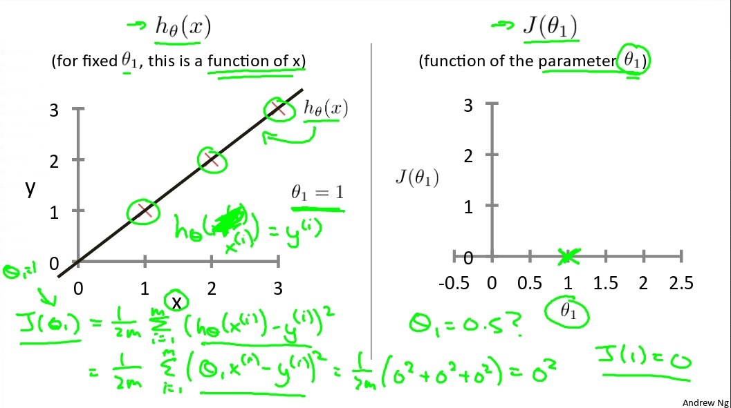
Hypothesis Function formula: $h_\theta(x) = \theta x$
Hypothesis Function is our predict function, x comes from the given data such as the size of the house, we need to find out θ to make this function work.
Cost Function formula: $J(\theta) = \frac{1}{2m}\sum\limits_{i=0}^m(h_\theta(x) - y)^2$
Relationship between hypothesis function and cost function
When cost function $J(\theta)$ gets its minimal value, then the θ is the exactly value which hypothesis function are looking for. In other words, cost function is a squared error function, it’s made up by many tiny errors between $h_\theta(x)$ and y, when all these tiny errors gets minimal, then the output value of hypothesis function $h_\theta(x)$ produced closely approximates y. After that we can use hypothesis function $h_\theta(x)$ to predict such as the price of the house. Here are a grap to show you the relationship between them:

Cost Function With Two Parameters

Hypothesis Function formula: $h_\theta(x) = \theta_0 + \theta_1x$
Cost Function formula: $J(\theta_0,\theta_1) = \frac{1}{2m}\sum\limits_{i=0}^m(h_\theta(x) - y)^2$

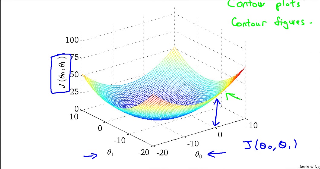
This time we need to find out values of $\theta_0,\theta_1$ when cost function $J(\theta_0,\theta_1)$ gets minimal. During two parameters, cost funcion becomes a three dimensions geometric figure, which look like a bowl-shape, consist of three axis: $J(\theta_0,\theta_1)$, $\theta_0$, $\theta_1$.

Relationship between hypothesis function and cost function in two parameters
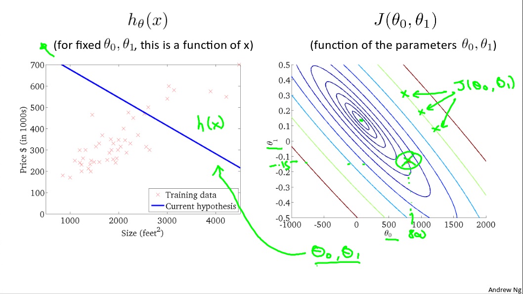
Right below is a contour plot, which consist of contour lines. A contour line of a two variable function has a constant value at all points of the same line. For example, These three green points found on the green line below have the same value for $J(\theta_0,\theta_1)$ and as a result, they are found along the same line. The circled x displays the value of the cost function for the grap on the left when $\theta_0$ = 800, and $\theta_1$ = -0.15.

Gradient Descent With One Parameter

Gradient descent is a way that cost function $J(\theta)$ used to get to its minimal value by steps.

Gradient descent formula: repeat $\theta = \theta - \alpha\frac{\partial}{\partial\theta}J(\theta)$
$\frac{\partial}{\partial\theta}J(\theta)$ is the slope of gradient, it could be positive or negative, but eventually it becomes 0 and $\theta$ would be stabilized on one value.

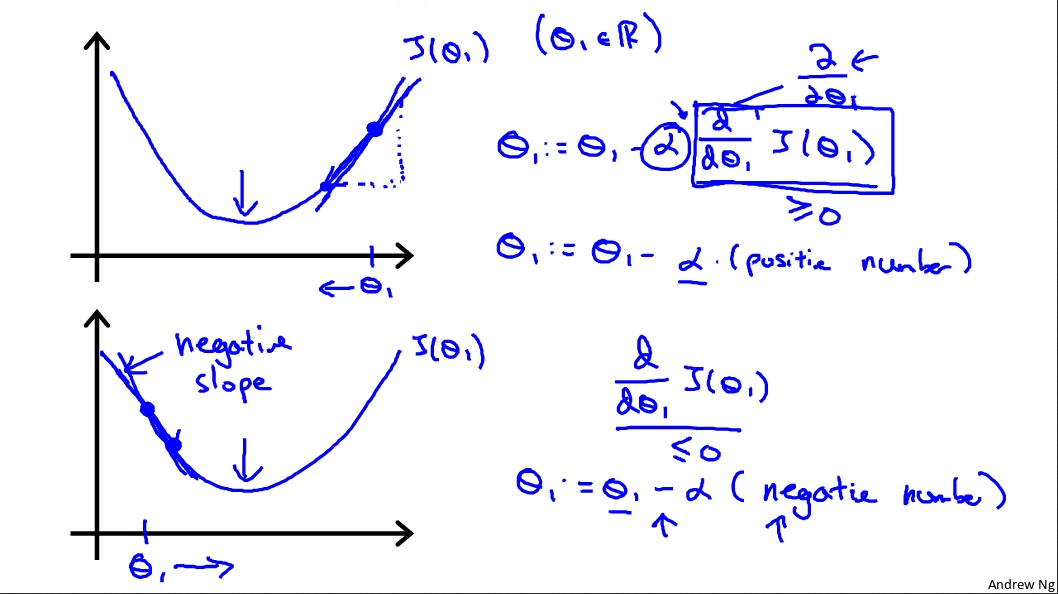
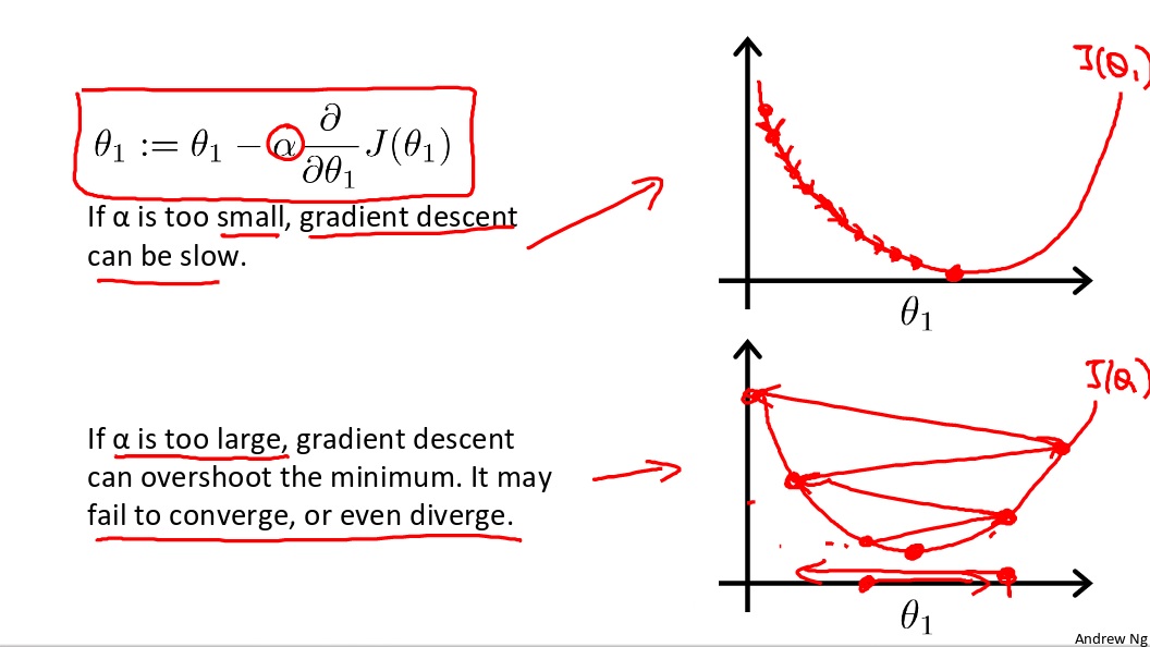
Picking that value of $\alpha$ is a technical skill. $\alpha$ is called learning rate, it can’t be too small or too large. When $\alpha$ is too small, gradient descent would taked longer to converge. When $\alpha$ is too large, it would caused overshoot problem, makes gradient descent fail to converge, or even diverge.

Gradient Descent With Two Parameters

Gradient descent formula: repeat $\theta_j = \theta_j - \alpha\frac{\partial}{\partial\theta}J(\theta_0,\theta_1)$

Gradient Descent For linear Regression

We substitute gradient descent and cost function below.

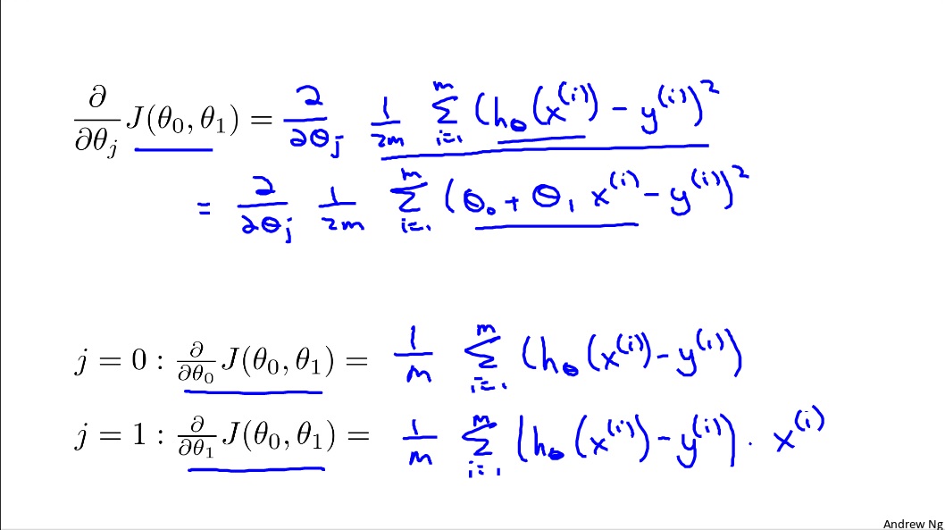
We update $\theta_0, \theta_1$ simultaneously.

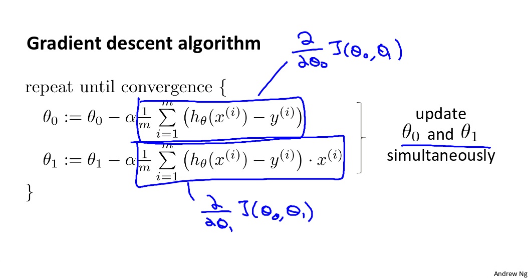
The point of all this is that if we start with a guess for our hypothesis and then repeatedly apply these gradient descent equations, our hypothesis will become more and more accurate.

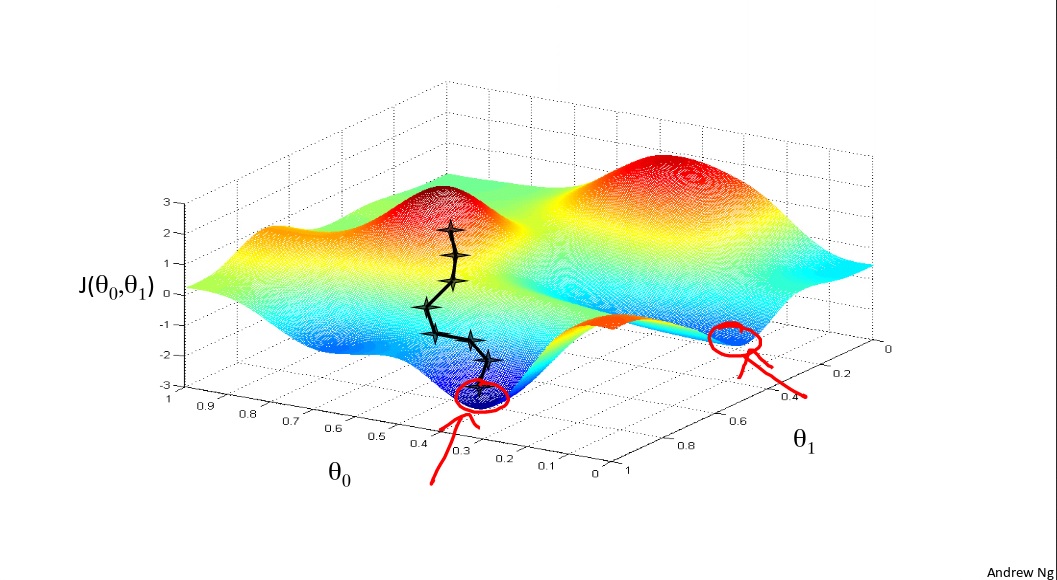
Local optima and global optima
Gradient descent would have a local optima problem. But for gradient descent for linear regression, it always gets the global optima, during it a convex function.

Note: All materials come from Coursera Andrew Ng’s Machine Learning Class.
Acknowledgement:
Coursera
Andrew Ng